Quick Start

This page will show some examples to load a sourced dataset or to make quicklook plots. For more details, please refer to the user manual.

More examples can be found here.

Use the Datahub and Dock a Dataset

The example below shows how to dock a sourced dataset (Madrigal/EISCAT data) to a datahub. Please refer to the list of the data sources for loading other geospace data.

Use the Time-Series Viewer and Create a Figure

Add Indicators

Use the Geomap Viewer and Create a Map

Use the Express Viewer and Create a Figure

The quicklook plots are produced by the method “quicklook” of a viewer, which is custom-designed for a data source. Those specialized viewer can be imported from geospacelab.express. The two examples below show the solar wind and geomagnetic indices, as well as the EISCAT data, respectively.

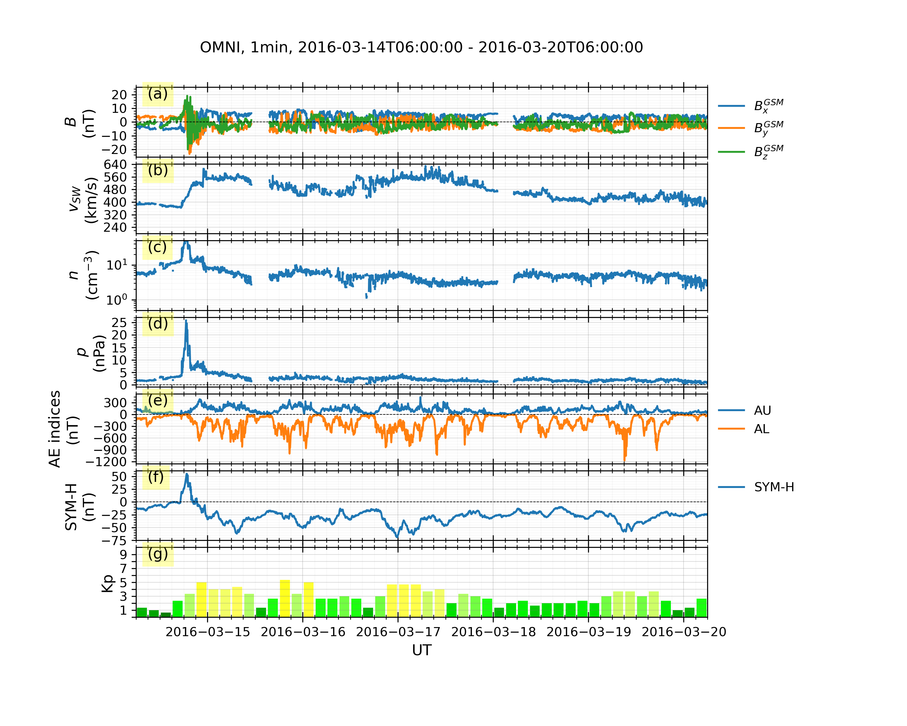
Solar Wind and Geomagnetic Indices from OMNI and WDC

Solar wind and geomagnetic indices data

examples/demo_omni_data.py

# Licensed under the BSD 3-Clause License
# Copyright (C) 2021 GeospaceLab (geospacelab)
# Author: Lei Cai, Space Physics and Astronomy, University of Oulu

__author__ = "Lei Cai"
__copyright__ = "Copyright 2021, GeospaceLab"
__license__ = "BSD-3-Clause License"
__email__ = "lei.cai@oulu.fi"
__docformat__ = "reStructureText"

import datetime
import geospacelab.express.omni_dashboard as omni

dt_fr = datetime.datetime.strptime('20160321' + '0600', '%Y%m%d%H%M')
dt_to = datetime.datetime.strptime('20160330' + '0600', '%Y%m%d%H%M')

omni_type = 'OMNI2'     # 'OMNI' or 'OMNI2'
omni_res = '5min'       # '1min' or '5min'
load_mode = 'AUTO'
dashboard = omni.OMNIDashboard(
    dt_fr, dt_to, omni_type=omni_type, omni_res=omni_res, load_mode=load_mode
)

# data can be retrieved in the same way as in Example 1:
dashboard.list_assigned_variables()
B_x_gsm = dashboard.get_variable('B_x_GSM', dataset_index=1)    # Omni dataset index is 1 in the OMNIDashboard. To check other dashboards, use the method "list_datasets()"
print(B_x_gsm)

dashboard.quicklook()

# save figure
dashboard.save_figure()

Output:

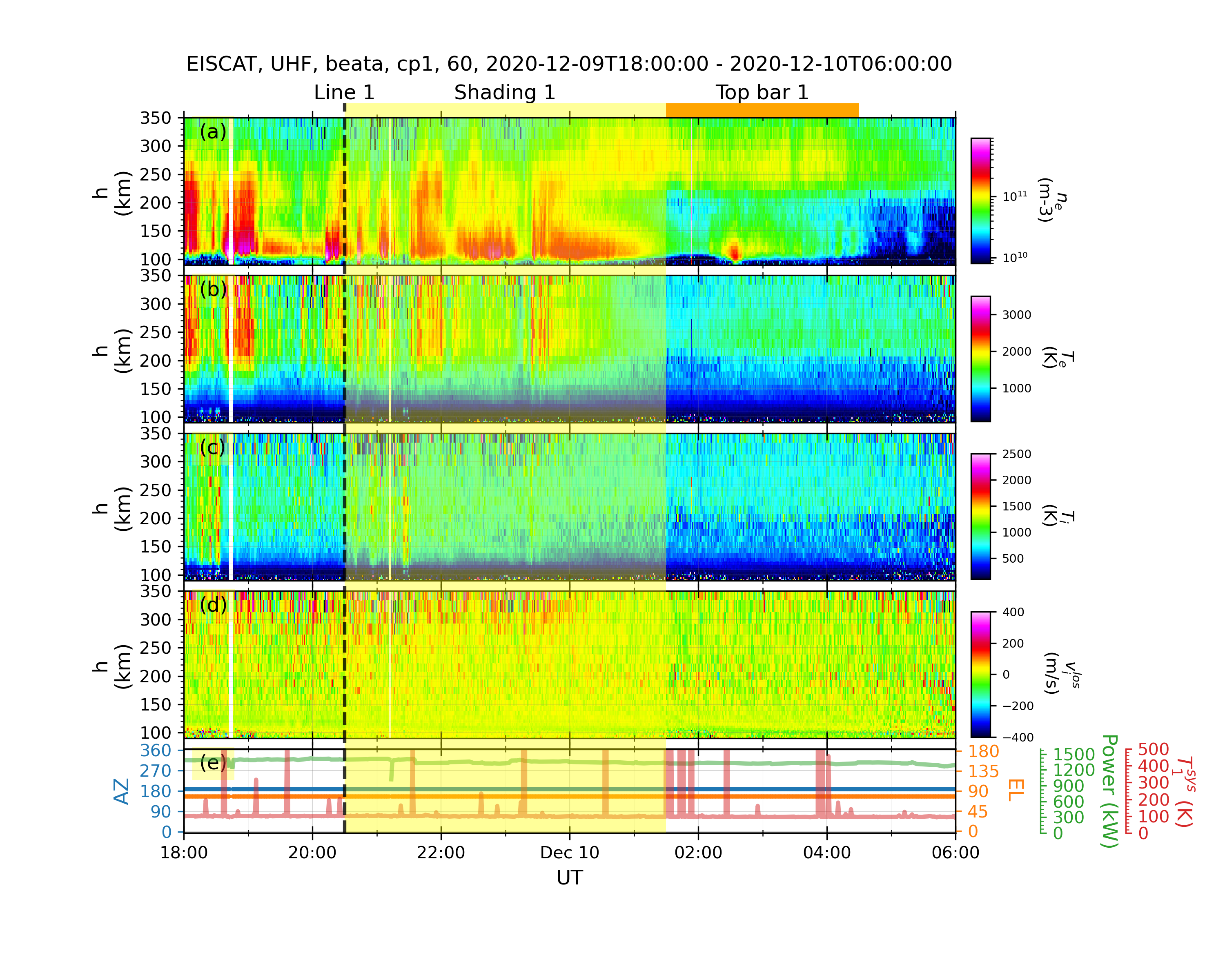
EISCAT from Madrigal with Marking Tools

examples/demo_eiscat_quicklook.py

# Licensed under the BSD 3-Clause License
# Copyright (C) 2021 GeospaceLab (geospacelab)
# Author: Lei Cai, Space Physics and Astronomy, University of Oulu

__author__ = "Lei Cai"
__copyright__ = "Copyright 2021, GeospaceLab"
__license__ = "BSD-3-Clause License"
__email__ = "lei.cai@oulu.fi"
__docformat__ = "reStructureText"

import datetime
import geospacelab.express.eiscat_dashboard as eiscat

dt_fr = datetime.datetime.strptime('20201209' + '1800', '%Y%m%d%H%M')
dt_to = datetime.datetime.strptime('20201210' + '0600', '%Y%m%d%H%M')

site = 'UHF'
antenna = 'UHF'
modulation = '60'
load_mode = 'AUTO'
dashboard = eiscat.EISCATDashboard(
    dt_fr, dt_to, site=site, antenna=antenna, modulation=modulation, load_mode='AUTO',
    data_file_type = "madrigal-hdf5"
)
dashboard.quicklook()

# dashboard.save_figure() # comment this if you need to run the following codes
# dashboard.show()   # comment this if you need to run the following codes.

"""
As the dashboard class (EISCATDashboard) is a inheritance of the classes Datahub and TSDashboard.
The variables can be retrieved in the same ways as shown in Example 1. 
"""
n_e = dashboard.assign_variable('n_e')
print(n_e.value)
print(n_e.error)

"""
Several marking tools (vertical lines, shadings, and top bars) can be added as the overlays 
on the top of the quicklook plot.
"""
# add vertical line
dt_fr_2 = datetime.datetime.strptime('20201209' + '2030', "%Y%m%d%H%M")
dt_to_2 = datetime.datetime.strptime('20201210' + '0130', "%Y%m%d%H%M")
dashboard.add_vertical_line(dt_fr_2, bottom_extend=0, top_extend=0.02, label='Line 1', label_position='top')
# add shading
dashboard.add_shading(dt_fr_2, dt_to_2, bottom_extend=0, top_extend=0.02, label='Shading 1', label_position='top')
# add top bar
dt_fr_3 = datetime.datetime.strptime('20201210' + '0130', "%Y%m%d%H%M")
dt_to_3 = datetime.datetime.strptime('20201210' + '0430', "%Y%m%d%H%M")
dashboard.add_top_bar(dt_fr_3, dt_to_3, bottom=0., top=0.02, label='Top bar 1')

# save figure
dashboard.save_figure()
# show on screen
dashboard.show()

Output:

DMSP/SSUSI auroral images

examples/demo_dmsp_ssusi_single_panel.py

import datetime
import matplotlib.pyplot as plt

# from geospacelab import preferences as pref
# pref.user_config['visualization']['mpl']['style'] = 'dark'
import geospacelab.visualization.mpl.geomap.geodashboards as geomap


def test_ssusi():
    dt_fr = datetime.datetime(2015, 9, 8, 8)
    dt_to = datetime.datetime(2015, 9, 8, 23, 59)
    time1 = datetime.datetime(2015, 9, 8, 20, 21)
    pole = 'N'
    sat_id = 'f16'
    band = 'LBHS'

    # Create a geodashboard object
    dashboard = geomap.GeoDashboard(dt_fr=dt_fr, dt_to=dt_to, figure_config={'figsize': (5, 5)})

    # If the orbit_id is specified, only one file will be downloaded. This option saves the downloading time.
    # dashboard.dock(datasource_contents=['jhuapl', 'dmsp', 'ssusi', 'edraur'], pole='N', sat_id='f17', orbit_id='46863')
    # If not specified, the data during the whole day will be downloaded.
    dashboard.dock(datasource_contents=['jhuapl', 'dmsp', 'ssusi', 'edraur'], pole=pole, sat_id=sat_id, orbit_id=None)
    ds_s1 = dashboard.dock(
        datasource_contents=['madrigal', 'satellites', 'dmsp', 's1'],
        dt_fr=time1 - datetime.timedelta(minutes=45),
        dt_to=time1 + datetime.timedelta(minutes=45),
        sat_id=sat_id, replace_orbit=True)

    dashboard.set_layout(1, 1)

    # Get the variables: LBHS emission intensiy, corresponding times and locations
    lbhs = dashboard.assign_variable('GRID_AUR_' + band, dataset_index=1)
    dts = dashboard.assign_variable('DATETIME', dataset_index=1).value.flatten()
    mlat = dashboard.assign_variable('GRID_MLAT', dataset_index=1).value
    mlon = dashboard.assign_variable('GRID_MLON', dataset_index=1).value
    mlt = dashboard.assign_variable(('GRID_MLT'), dataset_index=1).value

    # Search the index for the time to plot, used as an input to the following polar map
    ind_t = dashboard.datasets[1].get_time_ind(ut=time1)
    if (dts[ind_t] - time1).total_seconds()/60 > 60:     # in minutes
        raise ValueError("The time does not match any SSUSI data!")
    lbhs_ = lbhs.value[ind_t]
    mlat_ = mlat[ind_t]
    mlon_ = mlon[ind_t]
    mlt_ = mlt[ind_t]
    # Add a polar map panel to the dashboard. Currently the style is the fixed MLT at mlt_c=0. See the keywords below:
    panel1 = dashboard.add_polar_map(
        row_ind=0, col_ind=0, style='mlt-fixed', cs='AACGM',
        mlt_c=0., pole=pole, ut=time1, boundary_lat=55., mirror_south=True
    )

    # Some settings for plotting.
    pcolormesh_config = lbhs.visual.plot_config.pcolormesh
    # Overlay the SSUSI image in the map.
    ipc = panel1.overlay_pcolormesh(
        data=lbhs_, coords={'lat': mlat_, 'lon': mlon_, 'mlt': mlt_}, cs='AACGM', **pcolormesh_config)
    # Add a color bar
    panel1.add_colorbar(ipc, c_label=band + " (R)", c_scale=pcolormesh_config['c_scale'], left=1.1, bottom=0.1,
                        width=0.05, height=0.7)

    # Overlay the gridlines
    panel1.overlay_gridlines(lat_res=5, lon_label_separator=5)

    # Overlay the coastlines in the AACGM coordinate
    panel1.overlay_coastlines()

    # Overlay cross-track velocity along satellite trajectory
    sc_dt = ds_s1['SC_DATETIME'].value.flatten()
    sc_lat = ds_s1['SC_GEO_LAT'].value.flatten()
    sc_lon = ds_s1['SC_GEO_LON'].value.flatten()
    sc_alt = ds_s1['SC_GEO_ALT'].value.flatten()
    sc_coords = {'lat': sc_lat, 'lon': sc_lon, 'height': sc_alt}

    v_H = ds_s1['v_i_H'].value.flatten()
    panel1.overlay_cross_track_vector(
        vector=v_H, unit_vector=1000, vector_unit='m/s', alpha=0.3, color='red',
        sc_coords=sc_coords, sc_ut=sc_dt, cs='GEO',
    )
    # Overlay the satellite trajectory with ticks
    panel1.overlay_sc_trajectory(sc_ut=sc_dt, sc_coords=sc_coords, cs='GEO')

    # Overlay sites
    panel1.overlay_sites(site_ids=['TRO', 'ESR'], coords={'lat': [69.58, 78.15], 'lon': [19.23, 16.02], 'height': 0.}, cs='GEO', marker='^', markersize=2)

    # Add the title and save the figure
    polestr = 'North' if pole == 'N' else 'South'
    panel1.add_title(title='DMSP/SSUSI, ' + band + ', ' + sat_id.upper() + ', ' + polestr + ', ' + time1.strftime('%Y-%m-%d %H%M UT'))
    plt.savefig('DMSP_SSUSI_' + time1.strftime('%Y%m%d-%H%M') + '_' + band + '_' + sat_id.upper() + '_' + pole, dpi=300)

    # show the figure
    plt.show()


if __name__ == "__main__":
    test_ssusi()

Output: